| Assessing Floyd's Floods | ||||||||
|
The Flood team obtained data from three different satellites to measure the extent of the floods in North Carolina and to analyze sediment concentrations in the water. Each of the satellites has certain advantages and disadvantages. The NOAA Advanced Very High Resolution Radiometer (AVHRR) has wide spatial coverage, enabling it to see most of the Earth's surface every day. However, its resolution is relatively coarse-each pixel represents one square kilometer-so it was difficult to glean detailed information about the flood from AVHRR. To compensate, they used Landsat 7 and Radarsat, both of which provide much higher spatial resolution (up to 15 meters per pixel), but they revisit a given point on the surface much less frequently (about once every 8 days over eastern North Carolina). Some rivers can actually overrun their banks and then recede to near normal conditions between two consecutive Landsat and Radarsat acquisitions. |
||||||||

This flood map shows a comparison of the flood data collected by AVHRR (pink pixels), Radarsat (red pixels), and Landsat 7 (green pixels). These colors show areas that were flooded in the wake of Hurricane Floyd. Due to interference from clouds and forest canopies, geographers often get the best insight into a flood when they use data from multiple satellite sensors. (Image courtesy Dartmouth Flood Observatory, E. Anderson and R.H. Brakenridge) click to enlarge On September 17 and 18, 1999, AVHRR acquired clear shots of the floods, while Radarsat got its first look on September 23 and Landsat 7 obtained its first cloud-free image over eastern North Carolina on September 30. Because there were two major Hurricanes (Dennis and Floyd) within 11 days of one another, interspersed with heavy thundershowers, the ground was saturated and the floodwaters remained high during this entire period. Each satellite was able to capture valuable information about the ongoing event. Mertes points out that measuring flood extent is not as simple as merely counting pixels of water in an image and then adding up the totals. Much of the flooded areas can be hidden under dense vegetation canopies where they are hard to see. Radar data are particularly effective for detecting water under vegetation (Alsdorf et al. 2000), but are not effective for detecting water color. In contrast, because of its high spatial resolution and its sensitivity to certain wavelengths (colors) of light, the ETM+ aboard Landsat 7 enabled Mertes to detect water quality (with respect to sediment) in flooded areas. Combining data from each of these different instruments provides the most complete picture. Mertes explains that when sunlight hits water, some of it is immediately reflected by the surface back up into the air, and some of the light is refracted but penetrates beneath the surface, where some of it is absorbed and some is scattered by water and sediment particles. Some of the scattered light is reflected back up through the surface and up through the atmosphere. Satellite remote sensors can measure this "water-leaving radiance" (backscattered light). The more sediment particles there are in the water, the greater the amount of backscattered light. In short, whereas clear water appears dark in optical wavelengths because it tends to absorb most incoming sunlight, sediment-rich waters appear brighter because they reflect more sunlight. Mertes uses a computer program to quickly scan an entire satellite scene looking for both the darkest and the brightest water pixels. Because these two pixels represent the extremes of high and low reflectance values, she labels them as "endmembers" and then plots the reflectance of each pixel at a range of visible and near infrared wavelengths (from 400 to 900 nanometers). The reflectance values for all other pixels containing water will fall somewhere between her two endmembers, but will somewhat resemble their unique shapes, or "spectral signatures" (Mertes 1997). |
| |||||||
Next, Mertes begins to look for spectral signatures over regions that differ from her water endmembers. Those pixels with dramatically different reflectance curves can be identified as other surface features, such as land surface, concrete, or tree canopies. But those vegetated pixels with only slightly varying reflectance curves probably also contain some standing water. According to Mertes, the probability of there being water underlying the canopy is a function of how closely the reflectance curves match. Above a certain difference threshold, Mertes can flag those pixels that are purely vegetated surface and distinguish them from those that contain floodwater. Using this technique on the three major rivers that overran their banks in eastern North Carolina—the Neuse, Tar, and Roanoke Rivers—Mertes determined that a total of at least 790 square kilometers were flooded. Of that combined area, 520 square kilometers were clearly open water, while at least 270 were flooded vegetation. But could she tell how much sediment was contained in the runoff? Or, where the sediment came from? |
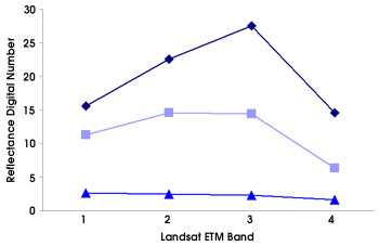
This graph shows typical endmember measurements that Leal Mertes uses to determine the amount of sediment suspended near the surface in a given body of water. The top and bottom lines show reflectance values for three different samples at each of four different wavelengths that correspond to four of Landsat 7's bands. The top and bottom lines are based upon measurements made from samples in the laboratory, with suspended sediment concentrations of 5.6 milligrams per liter (low) and 207 mg/L (high), respectively. The middle line shows reflectance values collected by Landsat over a body of water that contains an intermediate concentration of suspended sediment. (Graph courtesy Leal Mertes) 
|
|||||||
